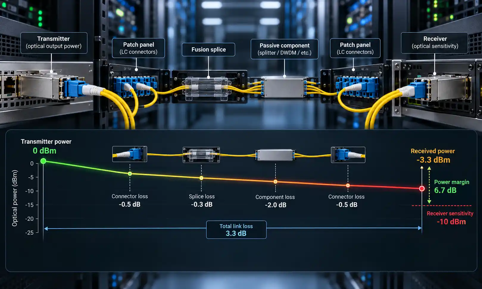
A fiber link is feasible only when the optical loss through the real cable path stays within the operating limits of the selected transmitter and receiver. The calculation should therefore compare two sides of the link: how much optical loss the active equipment can tolerate, and how much loss the installed fiber path is expected to introduce.
The basic relationships are:
Available power budget = minimum transmitter power − receiver sensitivity
Estimated link loss = fiber loss + connector loss + splice loss + other passive losses
Remaining power margin = available power budget − estimated link loss
A positive margin is an important first check, but it is not the whole design. The link must also satisfy the transceiver's fiber type, wavelength, reach, channel insertion-loss limit, dispersion requirements, and maximum receive-power limit. That last point matters because an optical link can fail from too little received power, while some short links using high-power long-reach optics can also overload the receiver.
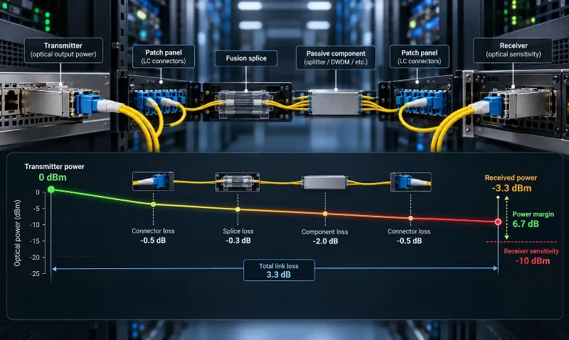
Fiber Optic Link Budget
Before installation, collect the optical specifications of the actual transceiver and map every passive element in the route. At minimum, identify:
- Minimum guaranteed transmitter power
- Receiver sensitivity
- Maximum receive power, when specified
- Maximum channel insertion loss, when specified
- Fiber type, wavelength, route length, and attenuation
- Every mated connection, splice, cassette, splitter, attenuator, or other passive device
- The engineering margin required by the project, manufacturer, or applicable standard
Use those values to calculate the worst-case power budget and the expected passive-path loss. If the application or transceiver documentation provides a stricter channel-loss limit than a simple Tx-to-Rx calculation, the stricter limit should control the design.
Power Budget and Link Loss Budget Are Different
Many link-budget mistakes start by treating these two quantities as interchangeable. They are related, but they describe different sides of the same optical path.
Optical Power Budget
The optical power budget describes how much signal loss the transmitter and receiver can tolerate together. For worst-case planning:
Power Budget (dB) = Minimum Tx Power (dBm) − Receiver Sensitivity (dBm)
Use the guaranteed minimum Tx value rather than a typical or maximum output value. Juniper's fiber-optic power-budget planning guidance uses this same worst-case approach: minimum transmitter power is compared with minimum receiver sensitivity before link loss is subtracted.
When selecting fiber optic transceivers, do not rely on the nominal distance printed in a product name alone. The Tx and Rx limits in the actual optical specification are the numbers that matter for a link-budget calculation.
Cable Plant Loss Budget
The cable plant loss budget estimates how much optical power the passive path will consume. It may include:
- Fiber attenuation
- Mated connector loss
- Fusion or mechanical splice loss
- Patch panels and adapters
- MPO/MTP cassettes and breakout assemblies
- PLC splitters or wavelength-selective components
- Fixed optical attenuators
- Other passive devices in the signal path
The general relationship is:
Estimated Link Loss = Fiber Loss + Connection Loss + Splice Loss + Other Passive Loss
This number describes the physical cable plant. It is not the same as the active equipment's available power budget.
Remaining Power Margin
Once both sides are known:
Remaining Margin = Available Power Budget − Estimated Link Loss
The remaining margin is the optical headroom left before the received signal reaches the lower operating limit used in the calculation. A project may reserve some of that headroom for component variation, measurement uncertainty, future reconfiguration, repair splices, contamination, aging, or environmental change.
Do not apply one fixed margin value to every network. Use the requirement defined by the project specification, equipment documentation, or applicable engineering standard.
How to Read the Transceiver Datasheet Before You Calculate
A reliable link budget begins with the actual optical specification, not with a generic internet value. The key rows in a transceiver datasheet usually include minimum Tx power, maximum Tx power, receiver sensitivity or minimum receive power, maximum receive power, wavelength, and sometimes a defined channel insertion-loss limit.
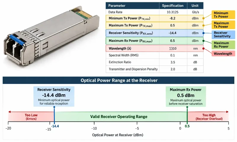
Minimum Transmitter Power
Minimum Tx power is the conservative starting point for checking whether enough light can reach the far-end receiver. A module can operate anywhere within its specified output range, so using typical or maximum output can make a marginal link look healthier than its guaranteed worst-case condition.
Receiver Sensitivity
Receiver sensitivity defines the low-power boundary used for the power-budget calculation. When minimum Tx and receiver sensitivity are both expressed in dBm, subtracting them gives a difference in dB.
Maximum Receive Power
Maximum receive power defines the upper optical input boundary. Cisco's 10GBASE SFP+ module data sheet lists both minimum and maximum transmit and receive levels for supported optics. It also documents overload considerations for high-power long-reach modules, which is why a short optical path cannot be approved only by checking receiver sensitivity.
This is especially relevant when reviewing long-reach SFP transceivers for a much shorter installed route.
Maximum Channel Insertion Loss
If the Ethernet application or transceiver documentation specifies a maximum channel insertion loss, treat that as an application limit rather than assuming the full Tx-to-Rx difference can be consumed by connectors and fiber.
At higher data rates, link reach can also be constrained by dispersion, modulation penalties, reflectance, lane architecture, FEC requirements, or other parameters that a simple optical-power subtraction does not represent.
What Passive Losses Need to Be Counted?
Fiber Attenuation
Fiber attenuation is normally specified in dB per kilometer at a particular wavelength:
Fiber Loss = Fiber Length × Attenuation Coefficient
Use the value for the actual fiber, wavelength, cable specification, and project requirement. A 1310 nm link should not be calculated with an attenuation figure that applies only at another wavelength.
For a short data-center channel, connectors and cassettes may consume a larger share of the total budget than the fiber itself. On a long outside-plant single-mode route, fiber attenuation may become one of the dominant terms.
Mated Connections
Count the complete optical path rather than only the long cable run. A rack-to-rack link may pass through adapters, patch panels, cross-connects, and short jumpers that are easy to overlook on a simplified network diagram.
If your calculation uses a loss value per mated pair, count mated interfaces according to the same method used by the manufacturer or project specification. Do not mix a per-connector value with a per-mated-pair count.
For standard LC, SC, FC, or other patching systems, the relevant assembly data should come from the actual fiber cable assemblies and connection components being specified.
Splices
Include every planned splice and distinguish between splice types when their allowed losses differ. A route with field repair points or intermediate closures may have more splice events than a basic network drawing suggests.
MPO/MTP Cassettes and High-Density Connections
Parallel-optics and high-density cabling can add several mating points, trunks, cassettes, and breakout assemblies to the channel. Do not assume that every MPO/MTP component has the same insertion-loss allowance.
When multiple MPO/MTP cable assemblies or cassettes are cascaded, calculate each specified loss individually. This is often more useful than treating the entire high-density path as one generic connector allowance.
Splitters, WDM Components, and Attenuators
Passive devices such as PLC splitters, filters, mux/demux units, optical taps, or fixed attenuators can introduce losses that are much larger than an ordinary mated connection. Use the specified insertion loss of the actual device.
An optical attenuator may also be intentionally required when the received optical level would otherwise exceed the receiver's permitted maximum.
How to Calculate a Fiber Optic Link Budget Step by Step
Step 1: Calculate the Worst-Case Optical Power Budget
Identify the minimum guaranteed Tx power and receiver sensitivity:
Power Budget = Minimum Tx − Receiver Sensitivity
Record any specified maximum channel insertion loss at the same time. If it is more restrictive than the raw Tx-to-Rx difference, use the stricter application limit.
Step 2: Calculate Fiber Attenuation
Measure or estimate the real route length, including planned routing and slack where applicable:
Fiber Loss = Length in km × Attenuation in dB/km
Step 3: Add Every Mated Connection
Count all relevant patch-panel, adapter, cross-connect, cassette, and equipment interfaces according to the counting method used by the specification:
Connection Loss = Number of Counted Connections × Allowed Loss per Connection
Step 4: Add Splice Loss
Splice Loss = Number of Splices × Allowed Loss per Splice
Use separate allowances if fusion and mechanical splices are treated differently in the project.
Step 5: Add Other Passive Components
Add the specified insertion loss for any splitter, WDM device, cassette, tap, attenuator, or other passive optical component.
Step 6: Add the Required Engineering Margin
Apply the margin required by the design specification or equipment documentation. A margin is an allowance for uncertainty and future change; it is not a substitute for accurate component data.
Step 7: Compare the Calculated Loss with the Permitted Limit
Estimated Link Loss + Required Margin ≤ Permitted Optical Loss
If this condition is not met, revise the design before installation. Options can include reducing unnecessary mating points, using lower-loss assemblies, shortening the route, changing the optical architecture, or selecting a transceiver with an appropriate link specification.
Step 8: Check the Receiver Overload Condition
When maximum receive power is specified, also estimate the highest possible received optical level:
Expected Maximum Rx Power = Maximum Tx Power − Minimum Expected Link Loss
The result should remain within the receiver's allowed input range. This check becomes particularly important when high-power, long-reach optics are installed on short fiber paths.
Worked Example: From Power Budget to Remaining Margin
A useful complete example appears in Juniper's official network cable and transceiver planning documentation. Juniper first calculates a 13 dB power budget from a minimum transmitter power of −15 dBm and receiver sensitivity of −28 dBm. It then applies that budget to a hypothetical 2 km multimode link.
| Item | Example Value | Calculated Loss |
|---|---|---|
| Available power budget | −15 dBm Tx and −28 dBm receiver sensitivity | 13 dB |
| Fiber attenuation | 2 km at 1 dB/km | 2 dB |
| Connectors | 5 at 0.5 dB each | 2.5 dB |
| Splices | 2 at 0.5 dB each | 1 dB |
| Higher-order mode loss | Example allowance | 0.5 dB |
| Total example link loss | 2 + 2.5 + 1 + 0.5 | 6 dB |
| Remaining power margin | 13 − 6 | 7 dB |

The value of this example is not that every project should use the same connector, splice, or fiber-loss figures. Juniper explicitly presents them as estimated values for its sample calculation and directs users to vendor documentation for actual equipment and component loss. The method is what should be carried into a real design:
Actual transceiver limits → actual route → actual component losses → required margin → final pass/fail decision
Why a Transceiver's Distance Rating Is Not Enough
A module labeled for 10 km, 20 km, 40 km, or another nominal reach does not mean every route shorter than that distance automatically meets the optical application.
Two links can have the same fiber distance but very different passive loss:
- A direct run with two mated connections and no intermediate splice
- The same distance routed through several patch panels, cross-connects, cassettes, and repair splices
The second route consumes more optical budget even though the geographic distance is unchanged.
The opposite problem also exists. A long-reach module used on a very short path may deliver more optical power than the receiver is intended to accept. Distance is therefore only one part of the link calculation.
When the Simple Tx-to-Rx Formula Is Not Enough
Minimum Tx − Receiver Sensitivity is a useful power-budget calculation, but it should not override a standardized application limit or transceiver-specific channel requirement.
Depending on the optical technology, the usable channel may also be constrained by:
- Modal or chromatic dispersion
- Transmitter and dispersion penalties
- Optical modulation requirements
- Reflectance
- Multi-lane optical architecture
- FEC-related application limits
This becomes increasingly important when planning 40G, 100G, 400G, and higher-speed links. In those systems, the transceiver's application specification should be treated as the final authority rather than assuming every dB between Tx and receiver sensitivity is available to the passive cabling.
How to Verify the Link After Installation
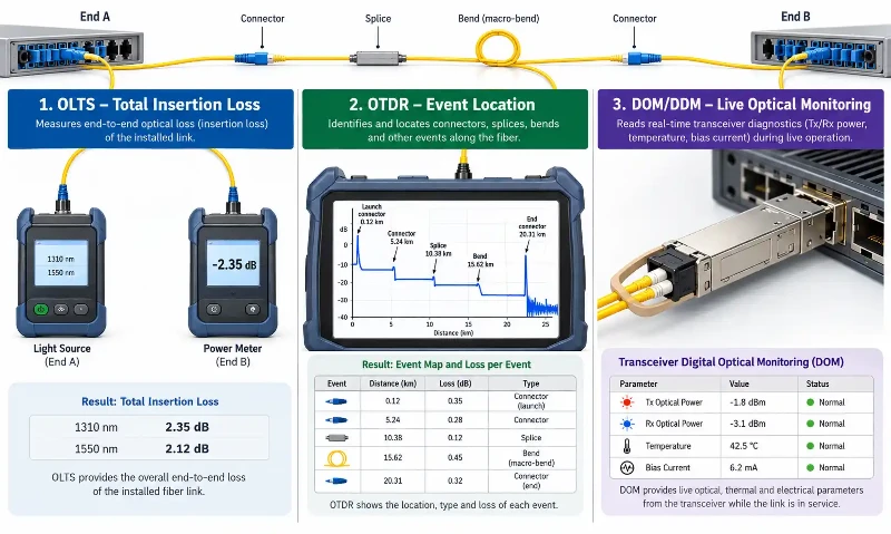
A link-budget calculation predicts what the installed path should support. Acceptance testing verifies what was actually built.
Use OLTS for End-to-End Insertion Loss
An Optical Loss Test Set measures the total end-to-end insertion loss of the installed link. That result can be compared with the project's defined loss limit or application requirement.
Use OTDR to Locate Individual Loss Events
An OTDR characterizes events along the fiber route. It can help locate high-loss connections, splice problems, unexpected bends, reflective events, and undocumented connection points.
Fluke Networks' OLTS and OTDR testing guidance describes the two methods as complementary: OLTS verifies the total insertion loss, while OTDR helps identify where individual losses occur.
For field installation and troubleshooting, the site's fiber optic installation and testing tools provide a relevant next step after the design-stage calculation.
Use DOM/DDM as an Operating Check, Not a Certification Substitute
Supported optical modules can report operating information such as Tx power, Rx power, temperature, and bias current through DOM/DDM. Those readings are useful for live troubleshooting and trend monitoring, but they do not replace a defined installation acceptance test.
Common Fiber Link Budget Mistakes
Using Typical or Maximum Tx Power for Worst-Case Reach
A typical reading describes expected behavior, not the guaranteed lower output boundary. For conservative reach planning, use the minimum Tx value unless the applicable specification defines another method.
Confusing dB and dBm
dBm is an absolute optical power level. dB is a difference, loss, or gain. Tx and Rx levels are commonly listed in dBm; fiber, connector, splice, and system losses are expressed in dB.
Counting the Long Fiber Run but Missing Rack-Level Connections
Dense patching environments are where simple calculations often fail. A relatively short channel can still accumulate meaningful loss through several mated pairs, cassettes, cross-connects, or breakout assemblies.
Treating Every Connector as the Same Loss
Use the specification for the actual connector or assembly. Standard-loss and low-loss interfaces should not be assigned the same value without supporting data.
Using One Fixed Safety Margin Everywhere
Do not copy a generic margin into every design. The margin should follow the approved engineering requirement for that project and application.
Ignoring Receiver Overload
Receiver sensitivity checks only the low-power boundary. If the module also specifies maximum receive power, verify the upper boundary as well.
Assuming a Passed Calculation Guarantees a Passed Installation
The calculation assumes that the installed components match the design and perform within specification. Contamination, poor splices, excessive bends, wrong components, or undocumented route changes can increase the actual loss. Test the completed link.
Frequently Asked Questions
What is the difference between optical power budget and fiber loss budget?
The optical power budget describes how much signal loss the transmitter and receiver can tolerate. The fiber or cable-plant loss budget estimates how much loss the passive route will introduce. A valid design compares the two rather than treating them as the same number.
How much safety margin should a fiber link budget include?
There is no single margin that should be applied blindly to every link. Use the value required by the project specification, equipment documentation, applicable standard, and expected future changes.
Can a fiber link have too little loss?
Yes. If a high-power transmitter is connected over a very short, low-loss path, the received optical level can exceed the module's specified maximum. Check maximum receive power and use attenuation only when required by the equipment specification.
Does MPO/MTP cabling consume more optical budget?
It depends on the number of mating points, cassettes, breakout assemblies, and the insertion-loss specification of the actual components. A high-density MPO/MTP channel should be calculated component by component rather than assigned one generic loss value.
Can DOM/DDM replace OLTS testing?
No. DOM/DDM is useful for observing live transceiver Tx and Rx levels, while OLTS is used to verify the end-to-end insertion loss of the installed cable path against a defined test limit.
Final Takeaway
A reliable fiber optic link budget is not simply a fiber-distance calculation, and it is not simply Tx power minus receiver sensitivity.
The transceiver defines the optical operating boundaries. The installed cable plant determines how much of that budget is consumed. A complete pre-installation decision therefore asks:
Can the real fiber path, including every connection, splice, passive component, and required margin, stay within the optical limits of the selected transceiver without falling below receiver sensitivity or exceeding maximum receive power?
If the answer is yes and the application-specific channel requirements are also satisfied, the design is ready to move into installation. After installation, verify the result with the required optical test method rather than relying on the calculation alone.